You are about to embark on an exciting journey in NLP to implement end to end solution to solve business problem. In the end of this tutorial, the reader should be able to understand the concept of NLP, TF-IDF and to implement multiclass classification algorithm using python programming language.

---

Contents

1. What is NLP

2. Application of NLP

3. What is TF-IDF

4. What is multiclass classification

5. Importance of multiclass classification

6. Installing libraries

7. Objective of the project

8. Implementing Multiclass Classification

---

1. What is Natural Language Processing

Natural language processing is the term used to describe the process of using computer algorithms to identify key elements in human language and extract meaning from unstructured spoken or written text. In other words, NLP is a set of AI techniques designed to process human language. These techniques enable applications to recognize, process, analyze, and even generate natural human language.

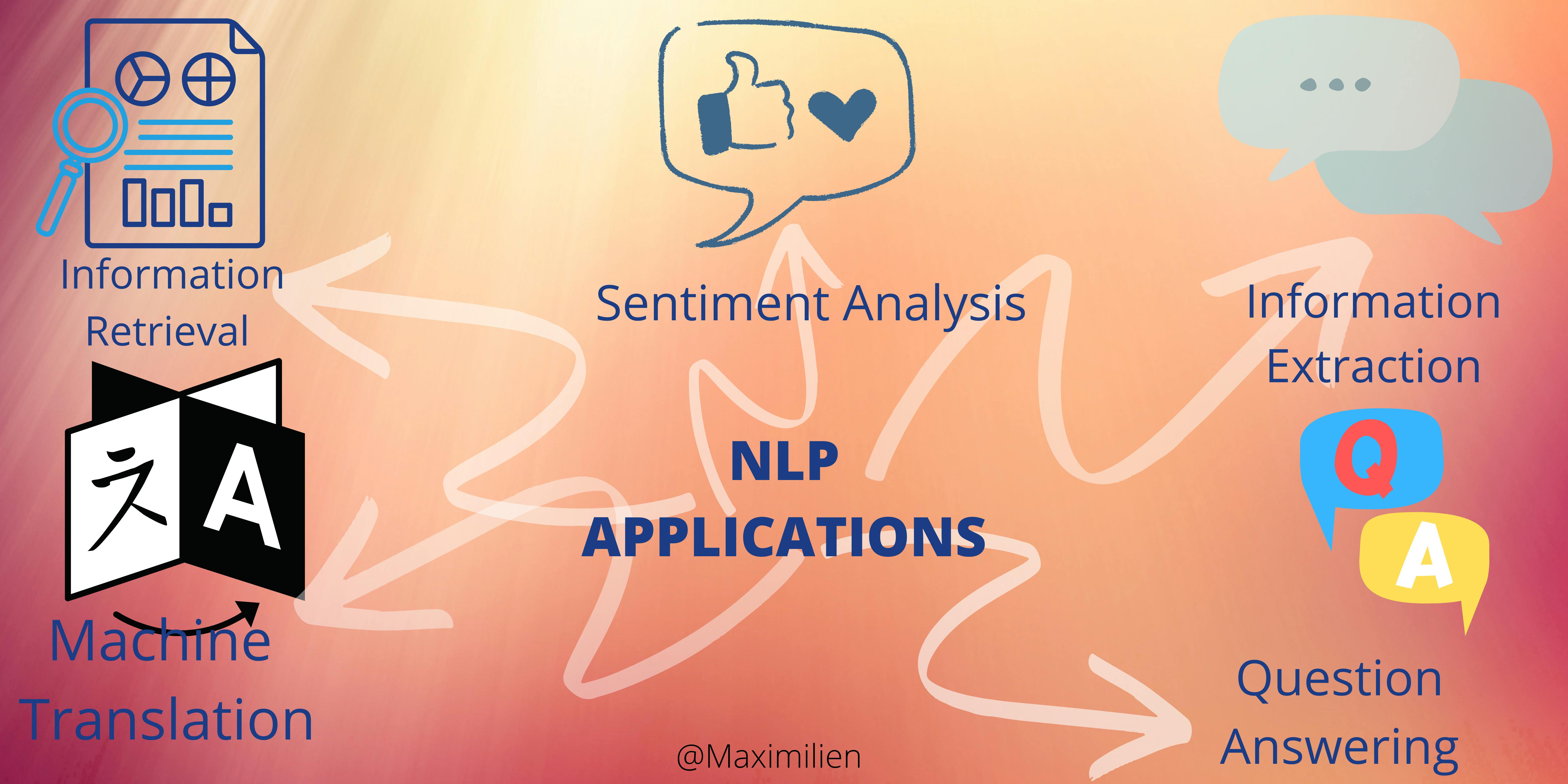
2. Application of NLP

3. What is TF-IDF

TD-IDF or term frequency-inverse document frequency is a Google algorithm used to score and rank a piece of content’s relevance to any given search query. It is used to check the occurrence of a keyword in a document and allocate importance to that keyword, based on the number of times it appears in the document. It also checks how relevant that keyword is across the web.

Mathematically speaking, in a context of term and document, TF is defined as the number of times a term appears in a document. Term and Document are independent variables and TF is dependent on these. Let us denote TF as a function of term (t) and document (d) : TF(t,d).

Moreover, In the context of term and all the documents in corpus, DF is defined as the number of documents that contain the term. Term and Document Corpus are independent variables and DF is dependent on these. Let us denote DF as a function of term (t) and document corpus (D) : DF(t,D).

NB: When the requirement is to calculate the importance of a term to a document in the corpus, TF denotes how important the term is to a document but it does not address the context of corpus. DF addresses how important a term in the context of a documents corpus. If a term appears across all documents, the term is overemphasized by TF. So the inverse of DF (IDF) could be used to project the actual importance of term, by calculating the product of TF and IDF.

Inverse of DF (IDF) formular: 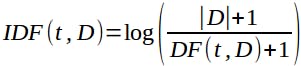With base of the log n > 1.

Product of TF and IDF formular:

Considering the following text corpus containing three documents below.

document1 : Welcome to maxtekIoT. There are many tutorials covering various fields of technology.

document2 : Technology has advanced a lot with the invention of semi-conductor transistor. Technology is changing our way of living.

document3 : You may find this tutorial on transistor technology interesting.

TFIDF(technology, document2, corpus)

TF(technology, document2) = 2

IDF(technology, document2) = log((3+1)/(3+1)) = 0

TFI-DF(technology, document2, corpus) = TF(technology, document2) . IDF(technology, document2) = 1 * 0 = 0

Conclusion: Though the term ‘technology’ appeared twice in document2 and the term has occurred in all the documents, it has no importance to document2 in the corpus.

4. What is multiclass classification

In machine learning, multiclass classification is an algorithm in which each feature in the dataset belongs to one of three or more classes in the dataset. So the aim of the algorithm is to construct a function in which given a new unseen feature point, the algorithm can precisely classify the class into which the new feature point belongs to.

5. Importance of multiclass classification

Multiclass classification enables a business analyst to predict which product a customer will purchase next from several options allowing the business to estimate expected revenue and adjust business practices and resources accordingly.

6. Installing libraries

in the following section till the end, all the codes should be written either in Jupyter notebook, Spyder or Google Colab. The following codes are written in Jupyter lab running on Debian 10 OS.

Various packages will be needed to be installed for the following code to execute if the reader is using Jupyter lab. To avoid this headache for newbies, we recommend you to use Google Colab cause most of the libraries and packages are preinstalled .

If you run through packages issues or libraries issues just type

!pip3 install name_of_the missing_package_pointing_to

7. Objective of the project

The goal of the project is to classify consumers’ complaints about financial products and services to companies for a response. Since it has multiple categories, it becomes a multiclass classification that can be solved through many of the machine learning algorithms. Once the algorithm is in place, whenever there is a new complaint, we can easily categorize it and can then be redirected to the concerned person. This will save a lot of time because we are minimizing the human intervention to decide whom this complaint should go to.

• Step 1 Importing the libraries

from sklearn import model_selection, preprocessing, metrics
from sklearn.feature_extraction.text import TfidfVectorizer
from sklearn.model_selection import StratifiedShuffleSplit
from sklearn.metrics import confusion_matrix
from nltk.corpus import stopwords
from collections import Counter
import matplotlib.pyplot as plt
from sklearn.svm import SVC
from textblob import Word
import seaborn as sns
import pandas as pd
import numpy as np

• Step 2 Loading the dataset read_csv() method from pandas library

df = pd.read_csv("consumer_complaints.csv")

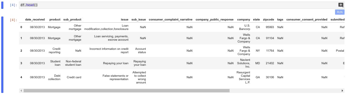
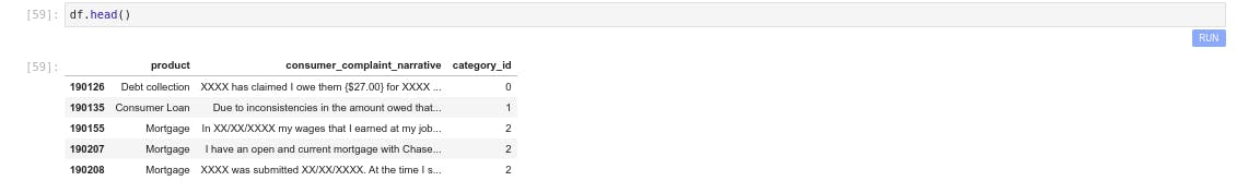
• Step 3 Exploratory data analysis Displaying the first five raw of the dataset

df.head()

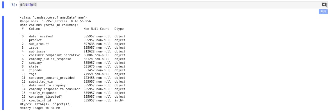
Displaying information about the data type and name of all the variables in the feature sets

df.info()

Adding category_id to the dataframe.(category_id shows which class each feature belongs to)

df['category_id'] = df['product'].factorize()[0]

We are only interesting in the product and the customer_complaint_narative all the rest of the feature sets are additional information which do not affect our analysis therefore they can be ignored.

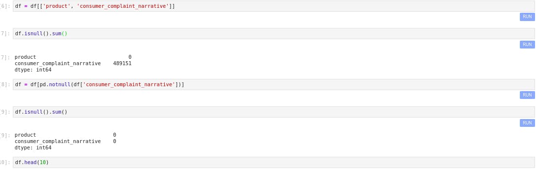
df = df[['product', 'consumer_complaint_narrative']]

Checking for NaN values in the dataframe

df.isnull().sum()

Keeping only no null values in the dataframe

df = df[pd.notnull(df['consumer_complaint_narrative'])]

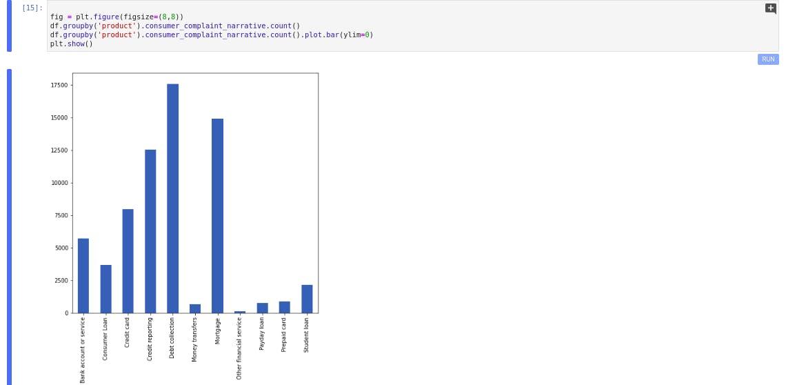
Grouping the product based on consumer_complaint_narrative and displaying the distribution

df.groupby('product').consumer_complaint_narrative.count()

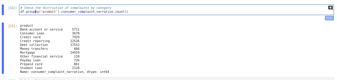
fig = plt.figure(figsize=(16,12))
df.groupby('product').consumer_complaint_narrative.count()
df.groupby('product').consumer_complaint_narrative.count().plot.bar(ylim=0)
plt.show()

• Step 4 Feature engineering using TF-IDF

Splitting the features into independent and dependent variables.

X=df['consumer_complaint_narrative']
y=df['product']

We did not use train_test_split to split the feature and target variables into train and test because. We noticed with train_test_split, the data were not proportionally distributed between y_train and y_test i.e some features appeared in the y_test only and not in the y_train. To fix that issue, we switched from train_test_split to StratifiedShuffleSplit.

n_splits = 1 # We only want a single split in this case
sss = StratifiedShuffleSplit(n_splits=n_splits, test_size=0.25, random_state=0)
for train_index, test_index in sss.split(X, y):
    X_train,X_test =X.iloc[train_index],X.iloc[test_index]
    y_train,y_test =y.iloc[train_index],y.iloc[test_index]

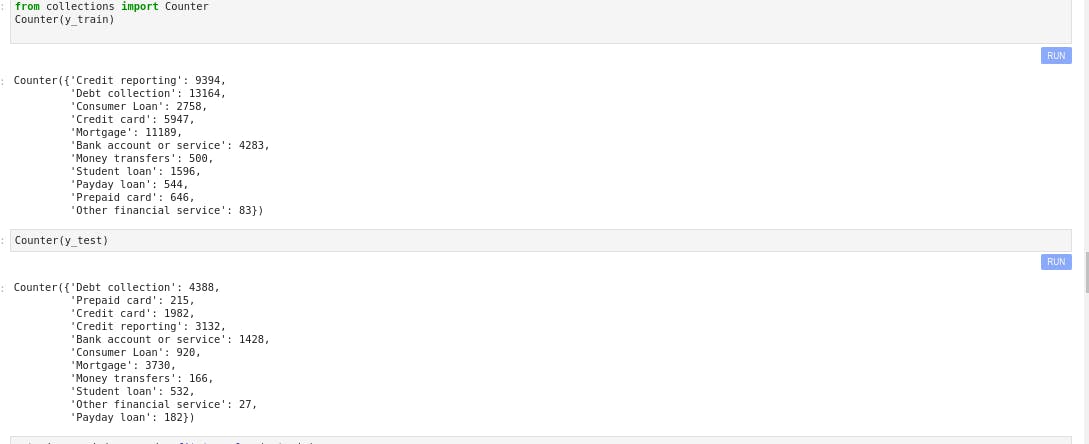
Checking the distribution of y_train and y_test

Counter(y_train)

Counter(y_test)

Encoding target variable. We fit_trainform() y_train and transform y_test

encoder = preprocessing.LabelEncoder()
y_train_encoded = encoder.fit_transform(y_train)
y_test_encoded = encoder.transform(y_test)

We initialized the TfidfVectorizer we had previously imported. After initializing ,we passed our data to the vectorizer and it transforms the data to a TF-IDF vector a matrix of array which is the mathematical representation of the corpus. This is done by using the fit_transform method.

vectorizer = TfidfVectorizer(analyzer='word',token_pattern=r'\w{1,}', max_features=5000)
tfidf_matrix=vectorizer.fit_transform(X)
tfidf_train=vectorizer.transform(X_train)
tfidf_train=vectorizer.transform(X_train)

if we want to observe the mathematical representation of our text i.e. the TF-IDF representation we have to convert the sparse matrix to a dense matrix. This is done by using the toarray() method

feature_array = tfidf_matrix.toarray()
feature_array

-Step 5 Model building and evaluation

model = SVC(C= .1, kernel='linear', gamma= 1)
model.fit(tfidf_train, y_train_encoded )
y_prediction=model.predict(tfidf_test)
accuracy = metrics.accuracy_score(y_prediction,y_test_encoded)
print ("Accuracy: ", accuracy)

Accuracy: 0.8164890432283559

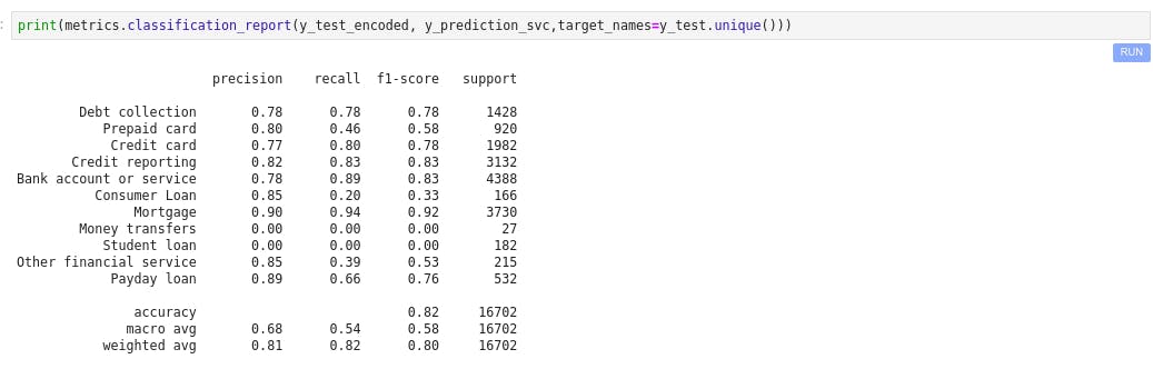
Classification report

print(metrics.classification_report(y_test_encoded, y_prediction,target_names=y_test.unique()))

Confusion matrix

conf_mat = confusion_matrix(y_test_encoded, y_prediction)
category_id_df = df[['product', 'category_id']].drop_duplicates().sort_values('category_id')
category_to_id = dict(category_id_df.values)
id_to_category = dict(category_id_df[['category_id','product']].values)
fig, ax = plt.subplots(figsize=(12,12))
sns.heatmap(conf_mat, annot=True, fmt='d', cmap="BuPu",xticklabels=category_id_df[['product']].values,yticklabels=category_id_df[['product']].values)
plt.ylabel('Actual')
plt.xlabel('Predicted')
plt.show()

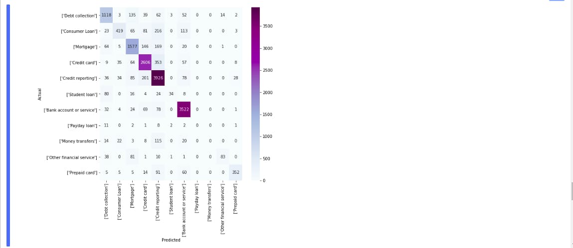
The accuracy of 82% is good for a baseline model. Precision and recall look pretty good across the categories except for “Payday loan.” If you look through Payload loan, most of the wrong predictions are Debt collection and Credit card, which might be because of the smaller number of samples in that category. It look like it’s a subcategory of a credit card. We can add these samples to any other group to make the model more stable.

-Step 6 Predicting unseen consumer complaint

corpus= ["This company refuses to pay my interest to my bank account"]
corpus_features = vectorizer.transform(corpus)
predictions = model.predict(corpus_features)
print(corpus)
print("  - Predicted as: '{}'".format(id_to_category[predictions[0]]))

['This company refuses to pay my interest to my bank account']

Predicted as: 'Debt collection'

corpus = ["This company refuses to provide me verification and validation of debt per my right under the FDCPA. I do not believe this debt is mine."]
corpus_features = vectorizer.transform(corpus)
predictions =svc_model.predict(corpus_features)
print(corpus)
print("  \n Predicted as: '{}'".format(id_to_category[predictions[0]]))

['This company refuses to provide me verification and validation of debt per my right under the FDCPA. I do not believe this debt is mine.']

Predicted as: 'Credit reporting'

• Conclusion: We achieve the aim of our objective by classifying consumer complaint using TF-IDF and Support Vector Algorithm with 82% accuracy. This model can be used as a baseline model. To increase the accuracy, we can do reiterate the process with different algorithms like Random Forest, GBM, Naive Bayes deep learning techniques like RNN and LSTM. Besides, other techniques can be used such as hyper-parameter tuning to improve the model accuracy which are out of the scope of this tutorial.

Please let me know if you find any errors. I can be contacted via LinkedIn here

My regards,

Maximilien.